Digital Signal Processing

The Digital Signal Processing (DSP) of Alice prepares the signal for its transmission in the physical domain.

The protocol that was used to define our experiment is described here, and the DSP can then be described as the following tasks:

Generation of symbols according to a modulation;
Upsampling;
Filtering
Frequency shift;
Frequency multiplexing of pilots;
Synchronisation sequence;
Padding of zeros.

In the following we describe each operation and show each function of the qosst_alice.dsp module can be used to make the DSP.

Generating the symbols and the baseband sequence

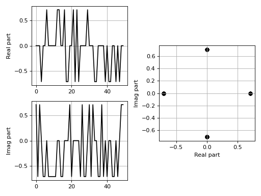
First we need to generate the baseband sequence and for this we can use the qosst_alice.dsp.generate_baseband_sequence() function. For this we must at least give the modulation we want to use, the variance, the size of the modulation (for discrete modulations) and the number of symbols we want.

There is a complete tutorial on the modulation on the qosst-core documentation, and here, for demonstrations purposes we will use a QPSK modulation (i.e. PSK modulation of size 4).

import matplotlib.pyplot as plt

from qosst_core.modulation import PSKModulation
from qosst_alice.dsp import generate_baseband_sequence

data = generate_baseband_sequence(
    modulation_cls=PSKModulation,
    variance=1,
    modulation_size=4,
    num_symbols=50,
)

fig, axs = plt.subplots(2, 2)
gs = axs[0, 1].get_gridspec()
for ax in axs[0:, -1]:
    ax.remove()
ax3 = fig.add_subplot(gs[0:, -1])
(ax, _), (ax2, _) = axs
ax.plot(data.real, color="black")
ax2.plot(data.imag, color="black")
ax3.scatter(data.real, data.imag, color="black")
ax3.set_aspect("equal")
ax.grid()
ax2.grid()
ax3.grid()
ax.set_ylabel("Real part")
ax2.set_ylabel("Imag part")
ax3.set_xlabel("Real part")
ax3.set_ylabel("Imag part")
fig.tight_layout()

(Source code, png, hires.png, pdf)

../_images/generate_baseband_sequence.png

Note

The number of symbols is low, for demonstration purposes.

Upsampling the data

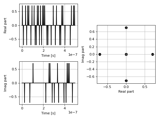
Next we upsample the data, the can be done with the qosst_alice.dsp.upsample() function. This is done because we are not sending the data at the same rate as the DAC. In practice we sent the data at a rate called the symbol rate \(R_S\) and the rate of the DAC is \(f_{DAC}\). The Samples-Per-Symbol (SPS) is defined as the ratio

\[\text{SPS} = \frac{f_{DAC}}{R_S}\]

and also happen to be the upsampling factor. For instance, if we send our data at 100 MSymbols/s (or equivalently 100MBaud) and the DAC has a rate of 500MSamples/s then SPS=5.

import matplotlib.pyplot as plt
import numpy as np

from qosst_core.modulation import PSKModulation
from qosst_alice.dsp import generate_baseband_sequence, upsample

data = generate_baseband_sequence(
    modulation_cls=PSKModulation,
    variance=1,
    modulation_size=4,
    num_symbols=50,
)

symbol_rate = 100e6
dac_rate = 500e6
sps = int(dac_rate / symbol_rate)

data = upsample(sequence=data, upsample_ratio=sps)

fig, axs = plt.subplots(2, 2)
gs = axs[0, 1].get_gridspec()
for ax in axs[0:, -1]:
    ax.remove()
ax3 = fig.add_subplot(gs[0:, -1])
(ax, _), (ax2, _) = axs
times = np.arange(len(data)) / dac_rate
ax.plot(times, data.real, color="black")
ax2.plot(times, data.imag, color="black")
ax3.scatter(data.real, data.imag, color="black")
ax3.set_aspect("equal")
ax.grid()
ax2.grid()
ax3.grid()
ax.set_xlabel("Time [s]")
ax2.set_xlabel("Time [s]")
ax.set_ylabel("Real part")
ax2.set_ylabel("Imag part")
ax3.set_xlabel("Real part")
ax3.set_ylabel("Imag part")
fig.tight_layout()

(Source code, png, hires.png, pdf)

Applying filter

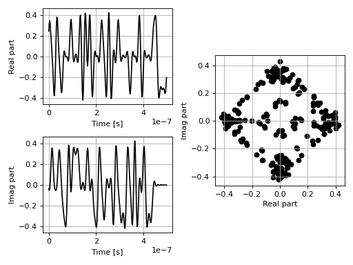
The next step is to apply a filter. The module offers two function: qosst_alice.dsp.apply_rrc_filter() and qosst_alice.dsp.apply_rectangular_filter() but here we focus on the first, since it’s more interesting for our scheme (and the one actually used).

The Raised-Cosine (RC) filter is a filter used for pulse-shaping that minimise inter-symbols interference. Its frequency response is defined as

\[\begin{split}H_{RC}(f) = \begin{cases} 1, & |f| \leq \frac{1 - \beta}{2T_S} \\ \frac{1}{2}\left[1 + \cos\left(\frac{\pi T_S}{\beta}\left[|f| - \frac{1 - \beta}{2T}\right]\right)\right], & \frac{1 - \beta}{2T_S} < |f| \leq \frac{1 + \beta}{2T_S} \\ 0, & \text{otherwise} \end{cases}\end{split}\]

where \(0\leq \beta \leq 1\) is called the roll-off factor and \(T_S = \frac{1}{R_S}\) is the inverse of the symbol rate.

The roll-off factor controls in a way the smoothness of the frequency response, and also defines the bandwidth of the resulting signal since

\[B = R_S(1+\beta) \]

For instance, if \(R_S=100\)Mbaud and \(\beta=0.5\), the resulting signal will have a bandwidth of 150MHz.

In our case, we apply the Raised Cosine filter in two parts: one at the transmitter and one at the receiver, by applying the Root-Raised-Cosine (RRC) filter defined as

\[H_{rc}(f) = H_{rrc}(f)\cdot H_{rrc}(f) \]

import matplotlib.pyplot as plt
import numpy as np

from qosst_core.modulation import PSKModulation
from qosst_alice.dsp import generate_baseband_sequence, upsample, apply_rrc_filter

data = generate_baseband_sequence(
    modulation_cls=PSKModulation,
    variance=1,
    modulation_size=4,
    num_symbols=50,
)

symbol_rate = 100e6
dac_rate = 500e6
sps = int(dac_rate / symbol_rate)

data = upsample(sequence=data, upsample_ratio=sps)

roll_off = 0.5

data = apply_rrc_filter(
    sequence=data,
    length=10 * sps + 2,
    roll_off=roll_off,
    symbol_period=1 / symbol_rate,
    sampling_rate=dac_rate,
)

fig, axs = plt.subplots(2, 2)
gs = axs[0, 1].get_gridspec()
for ax in axs[0:, -1]:
    ax.remove()
ax3 = fig.add_subplot(gs[0:, -1])
(ax, _), (ax2, _) = axs
times = np.arange(len(data)) / dac_rate
ax.plot(times, data.real, color="black")
ax2.plot(times, data.imag, color="black")
ax3.scatter(data.real, data.imag, color="black")
ax3.set_aspect("equal")
ax.grid()
ax2.grid()
ax3.grid()
ax.set_xlabel("Time [s]")
ax2.set_xlabel("Time [s]")
ax.set_ylabel("Real part")
ax2.set_ylabel("Imag part")
ax3.set_xlabel("Real part")
ax3.set_ylabel("Imag part")
fig.tight_layout()

(Source code, png, hires.png, pdf)

Shift the data

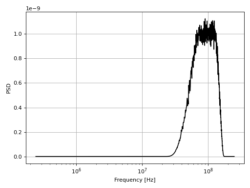
Next we want to shift our data in frequency to avoid low frequency noise. The only requirement for the value of \(f_shift\) is that the signal stays in the bandwidth of the detector and \(f_shift>\frac{B}{2}\) in case of a RF-heterodyne.

To shift the data, we can use the qosst_alice.dsp.frequency_shift() function.

import matplotlib.pyplot as plt
from scipy import signal
import numpy as np

from qosst_core.modulation import PSKModulation
from qosst_alice.dsp import (
    generate_baseband_sequence,
    upsample,
    apply_rrc_filter,
    shift_sequence,
)

data = generate_baseband_sequence(
    modulation_cls=PSKModulation,
    variance=1,
    modulation_size=4,
    num_symbols=100000,
)

symbol_rate = 100e6
dac_rate = 500e6
sps = int(dac_rate / symbol_rate)

data = upsample(sequence=data, upsample_ratio=sps)

roll_off = 0.5

data = apply_rrc_filter(
    sequence=data,
    length=10 * sps + 2,
    roll_off=roll_off,
    symbol_period=1 / symbol_rate,
    sampling_rate=dac_rate,
)

f_shift = 100e6

data = shift_sequence(
    sequence=data, frequency_shift_value=f_shift, sampling_rate=dac_rate
)

f, psd = signal.welch(data, fs=dac_rate, nperseg=2048)
mask = np.where(f > 0)[0]
fig, ax = plt.subplots(1, 1)
ax.semilogx(f[mask], psd[mask], color="black")
ax.set_xlabel("Frequency [Hz]")
ax.set_ylabel("PSD")
ax.grid()
fig.tight_layout()

(Source code, png, hires.png, pdf)

Note

We increased the number of symbols to be able to see a nice PSD.

Adding frequency multiplexing pilots

We then add frequency multiplexing pilots (usually 2) which are complex exponential

\[ pilot = \exp\left(2\pi i t f_{pilot}\right)\]

This can be done with the qosst_alice.dsp.add_frequency_multiplexed_pilots() function.

import matplotlib.pyplot as plt
from scipy import signal
import numpy as np

from qosst_core.modulation import PSKModulation
from qosst_alice.dsp import (
    generate_baseband_sequence,
    upsample,
    apply_rrc_filter,
    shift_sequence,
    add_frequency_multiplexed_pilots,
)

data = generate_baseband_sequence(
    modulation_cls=PSKModulation,
    variance=1,
    modulation_size=4,
    num_symbols=100000,
)

symbol_rate = 100e6
dac_rate = 500e6
sps = int(dac_rate / symbol_rate)

data = upsample(sequence=data, upsample_ratio=sps)

roll_off = 0.5

data = apply_rrc_filter(
    sequence=data,
    length=10 * sps + 2,
    roll_off=roll_off,
    symbol_period=1 / symbol_rate,
    sampling_rate=dac_rate,
)

f_shift = 100e6

data = shift_sequence(
    sequence=data, frequency_shift_value=f_shift, sampling_rate=dac_rate
)

pilots_frequencies = [200e6, 220e6]
pilots_amplitudes = [0.05, 0.05]

data = add_frequency_multiplexed_pilots(
    sequence=data,
    pilots_frequencies=pilots_frequencies,
    pilots_amplitudes=pilots_amplitudes,
    sampling_rate=dac_rate,
)

f, psd = signal.welch(data, fs=dac_rate, nperseg=2048)
mask = np.where(f > 0)[0]
fig, ax = plt.subplots(1, 1)
ax.semilogx(f[mask], psd[mask], color="black")
ax.set_xlabel("Frequency [Hz]")
ax.set_ylabel("PSD")
ax.grid()
fig.tight_layout()

(Source code, png, hires.png, pdf)

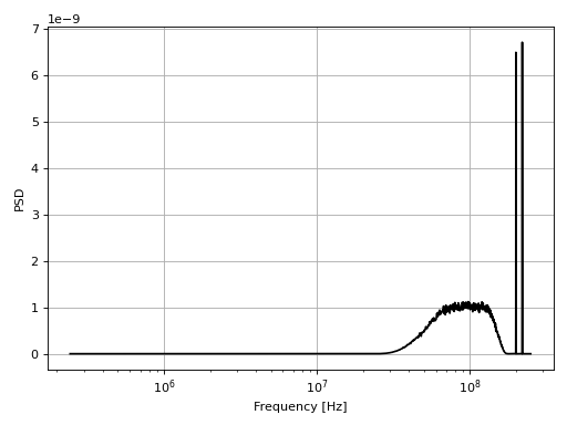
Note

Please note that the values used for the ratio and power of pilots are not good and are only those one for demonstration purposes.

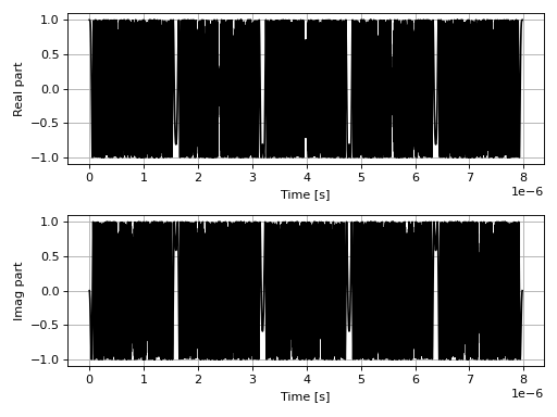
Adding a synchronisation sequence

We then add a synchronisation sequence. We use a Zadoff-Chu (ZC) sequence which is a CAZAC (Constant Amplitude Zero AutoCorrelation) sequence. In our case it is defined as

\[x_u(n)=\text{exp}\left(-i\frac{\pi un(n+1)}{N_{ZC}}\right)\]

for \(0\leq n \leq N_{ZC}\) where \(N_{ZC}\) is the length of the Zadoff-Chu sequence and \(u\) the root of the sequence, with the requirement that \(\text{gcd}(u, N_{ZC}) = 1\). In practice, we choose two prime numbers to ensure this condition.

This operation can be done with the qosst_alice.dsp.add_zc function.

import matplotlib.pyplot as plt
from scipy import signal
import numpy as np

from qosst_core.modulation import PSKModulation
from qosst_alice.dsp import (
    generate_baseband_sequence,
    upsample,
    apply_rrc_filter,
    shift_sequence,
    add_frequency_multiplexed_pilots,
    add_zc,
)

data = generate_baseband_sequence(
    modulation_cls=PSKModulation,
    variance=1,
    modulation_size=4,
    num_symbols=100000,
)

symbol_rate = 100e6
dac_rate = 500e6
sps = int(dac_rate / symbol_rate)

data = upsample(sequence=data, upsample_ratio=sps)

roll_off = 0.5

data = apply_rrc_filter(
    sequence=data,
    length=10 * sps + 2,
    roll_off=roll_off,
    symbol_period=1 / symbol_rate,
    sampling_rate=dac_rate,
)

f_shift = 100e6

data = shift_sequence(
    sequence=data, frequency_shift_value=f_shift, sampling_rate=dac_rate
)

pilots_frequencies = [200e6, 220e6]
pilots_amplitudes = [0.05, 0.05]

data = add_frequency_multiplexed_pilots(
    sequence=data,
    pilots_frequencies=pilots_frequencies,
    pilots_amplitudes=pilots_amplitudes,
    sampling_rate=dac_rate,
)

zc_root = 5
zc_length = 3989

data = add_zc(sequence=data, root=zc_root, length=zc_length)


fig, (ax, ax2) = plt.subplots(2, 1)
times = np.arange(len(data)) / dac_rate
ax.plot(times[:zc_length], data.real[:zc_length], color="black")
ax2.plot(times[:zc_length], data.imag[:zc_length], color="black")
ax.grid()
ax2.grid()
ax.set_xlabel("Time [s]")
ax2.set_xlabel("Time [s]")
ax.set_ylabel("Real part")
ax2.set_ylabel("Imag part")
fig.tight_layout()

(Source code, png, hires.png, pdf)

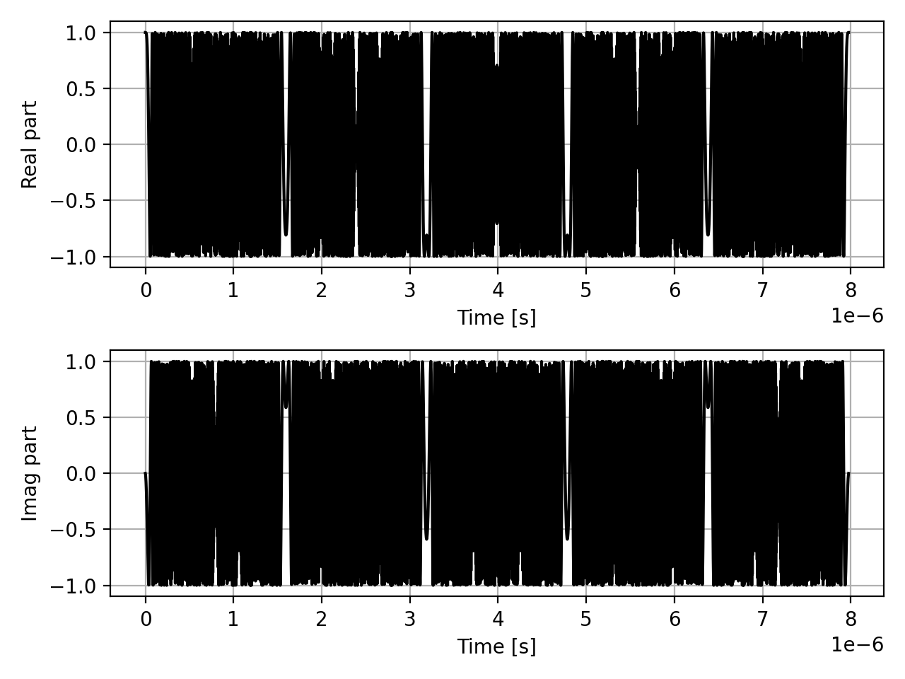
Padding zeros

Finally, in some cases we need to pad zeros at the beginning and end of the sequence. This can be done with the qosst_alice.dsp.add_zeros function.

import matplotlib.pyplot as plt
from scipy import signal
import numpy as np

from qosst_core.modulation import PSKModulation
from qosst_alice.dsp import (
    generate_baseband_sequence,
    upsample,
    apply_rrc_filter,
    shift_sequence,
    add_frequency_multiplexed_pilots,
    add_zc,
    add_zeros,
)

data = generate_baseband_sequence(
    modulation_cls=PSKModulation,
    variance=1,
    modulation_size=4,
    num_symbols=100000,
)

symbol_rate = 100e6
dac_rate = 500e6
sps = int(dac_rate / symbol_rate)

data = upsample(sequence=data, upsample_ratio=sps)

roll_off = 0.5

data = apply_rrc_filter(
    sequence=data,
    length=10 * sps + 2,
    roll_off=roll_off,
    symbol_period=1 / symbol_rate,
    sampling_rate=dac_rate,
)

f_shift = 100e6

data = shift_sequence(
    sequence=data, frequency_shift_value=f_shift, sampling_rate=dac_rate
)

pilots_frequencies = [200e6, 220e6]
pilots_amplitudes = [0.05, 0.05]

data = add_frequency_multiplexed_pilots(
    sequence=data,
    pilots_frequencies=pilots_frequencies,
    pilots_amplitudes=pilots_amplitudes,
    sampling_rate=dac_rate,
)

zc_root = 5
zc_length = 3989

data = add_zc(sequence=data, root=zc_root, length=zc_length)

data = add_zeros(sequence=data, num_zeros_start=int(zc_length / 2), num_zeros_end=0)

fig, (ax, ax2) = plt.subplots(2, 1)
times = np.arange(len(data)) / dac_rate
ax.plot(times[:zc_length], data.real[:zc_length], color="black")
ax2.plot(times[:zc_length], data.imag[:zc_length], color="black")
ax.grid()
ax2.grid()
ax.set_xlabel("Time [s]")
ax2.set_xlabel("Time [s]")
ax.set_ylabel("Real part")
ax2.set_ylabel("Imag part")
fig.tight_layout()

(Source code, png, hires.png, pdf)

The DSP function

The whole work we just did is encompassed in one, ready-to-use function, that is qosst_alice.dsp.dsp() and takes the whole configuration as a parameter.

Here is an example:

from qosst_core.configuration import Configuration
from qosst_alice.dsp import dsp_alice

config = Configuration("config.toml")

final, quantum_sequence, symbols = dsp_alice(config=config)

This is the code that is actually used in the qosst_alice.alice.QOSSTAlice._do_dsp() method to prepare the DSP of Alice.